Tutorial
In this tutorial, we will identify the splicing derived neoantigens (both MHC bound T antigens and altered surface B antigens) on the TCGA Skin Cutaneous Melanoma (SKCM) cohort (472 tumor samples).
Note
We will use the whole dataset (472 bam files) to demostrate the full functionalities of SNAF. Completing this tutorial will take several hours and requires a multi-core High Performance Compute environment (HPC). Please replace the bam file folder with yours and configure your sample HLA type file as illustrated below.
Warning
There are a few steps in the workflow that requires internet connection, especially when launching B-antigen viewer. To avoid any errors, it is recommended to make sure your system has internet connection, which shouldn’t be a problem for any computer or HPC.
Running AltAnalyze to identify alternative splicing events
The analysis starts with a group of bam files, with each BAM corresponding to single patient sample. For example, if you have all the bam files stored in /user/ligk2e/bam,
Please make sure you are in /user/ligk2e and run the following code:
# using docker
# -v mount the current folder to the /mnt folder in docker system, so that docker can access your bam folder
# first argument is the running mode, we set to "identify"
# second argument is the bam folder, we set to "bam"
# the third argument is the number of cores to use, we set to 4
docker run -v $PWD:/mnt -t frankligy123/altanalyze:0.7.0.1 identify bam 4

# if using singularity, you may have to use singularity/3.1 if you run into any error
singularity run -B $PWD:/mnt --writable altanalyze/ identify bam 4
Warning
1. What if you only have one bam file? Our original Altanalyze codebase was designed for cohort-level splicing analysis (so at least 2 samples). As a workaround, a quick fix is to copy your bam file to another one (sample.bam, sample_copy.bam), put them all in a folder, then run the pipeline.
Make sure there are no existing folders named
/bedand/altanalyze_outputin the same level of your/bamfolder.For your bam file, make sure no
__(double underscore) is present as this is a preserved delimiter in the program, just rename it
The output of this step contains different useful readouts, including splicing junction quantification, splicing event quantification and gene expression, but the most important output that will be used
in the following step is the junction count matrix. The junction count matrix will be the altanalyze_output/ExpressionInput/counts.original.pruned.txt. Let us take a look at a subsampled junction count matrix, each row represent a splicing junction
annotated by the AltAnalyze gene model, and each column represents the sample name. The numerical value represents the number of reads that support the
occurence of a certain junction.
Note
In altanalyze/ExpressionInput folder, you will find counts.original.full.txt and counts.original.pruned.txt, the former is the splicing junction whereas the latter
is the alternative splicing events. The latter can better filter out those constitutive junctions (if exon2-exon3 always occur it is a constitutive junction instead of alternative splicing
event). We recommend using the latter, but when you only have few samples (n<10), using the former can increase the sensitivity.
TCGA-EB-A82B-01A-11R-A352-07.bed |
TCGA-GF-A4EO-06A-12R-A24X-07.bed |
TCGA-D3-A1Q8-06A-11R-A18T-07.bed |
TCGA-FS-A1YY-06A-11R-A18T-07.bed |
TCGA-WE-A8ZM-06A-11R-A37K-07.bed |
TCGA-WE-A8ZN-06A-11R-A37K-07.bed |
TCGA-FW-A3TV-06A-11R-A239-07.bed |
TCGA-XV-AAZV-01A-11R-A40A-07.bed |
TCGA-DA-A1I1-06A-12R-A18U-07.bed |
TCGA-ER-A2NC-06A-11R-A18T-07.bed |
|
|---|---|---|---|---|---|---|---|---|---|---|
ENSG00000156398:E29.4-E31.1 |
1 |
1 |
0 |
2 |
3 |
0 |
3 |
0 |
2 |
3 |
ENSG00000095585:E8.1-E9.1 |
11 |
35 |
15 |
11 |
0 |
1 |
6 |
27 |
22 |
65 |
ENSG00000131069:E6.3-E10.2 |
39 |
99 |
98 |
71 |
64 |
9 |
86 |
49 |
77 |
34 |
ENSG00000171132:E14.1-E15.1 |
12 |
3 |
13 |
1 |
6 |
0 |
13 |
1 |
3 |
2 |
ENSG00000010278:E4.1-E6.1 |
69 |
5 |
146 |
149 |
54 |
27 |
47 |
68 |
13 |
26 |
ENSG00000214944:E40.1-E41.1 |
1 |
1 |
6 |
10 |
1 |
0 |
1 |
2 |
0 |
2 |
ENSG00000179912:E20.5-E27.1_57422959 |
0 |
2 |
4 |
2 |
0 |
0 |
2 |
0 |
2 |
3 |
ENSG00000186642:E9.2-E10.1 |
2 |
0 |
6 |
2 |
13 |
1 |
2 |
2 |
4 |
2 |
ENSG00000137497:E28.1-E29.1 |
265 |
110 |
95 |
221 |
349 |
157 |
200 |
111 |
221 |
115 |
ENSG00000114982:E22.1-E24.2 |
68 |
45 |
71 |
112 |
75 |
17 |
106 |
24 |
96 |
114 |
Note
In the future, we are planning to support user-supplied splicing count matrices from alternative algorithms, which will increase the compatability of the pipeline with other workflows.
Identify MHC-bound neoantigens (T-antigen)
With the junction count matrix, we can proceed to predict MHC-bound neoantigens (T antigen). The only additional input we need is
the patient HLA type information, in this analyis, we use Optitype to infer the 4 digit HLA type from RNA-Seq data, the sample_hla.txt file
looks like below example, please be compliant with the HLA format here:
            sample                                                  hla
TCGA-X1-A1WX-06A-11R-A38C-07.bed    HLA-A*02:01,HLA-A*02:01,HLA-B*39:10,HLA-B*15:01,HLA-C*03:03,HLA-C*12:03
TCGA-X2-A1WX-06A-11R-A38C-07.bed    HLA-A*02:01,HLA-A*01:01,HLA-B*40:01,HLA-B*52:01,HLA-C*03:04,HLA-C*12:02
TCGA-X3-A1WX-06A-11R-A38C-07.bed    HLA-A*11:01,HLA-A*32:01,HLA-B*40:02,HLA-B*35:01,HLA-C*04:01,HLA-C*02:02
TCGA-X4-A2PB-01A-11R-A18S-07.bed    HLA-A*02:01,HLA-A*01:01,HLA-B*07:02,HLA-B*18:01,HLA-C*07:01,HLA-C*07:02
Note
Optitype is again a tool that is super easy to install as they provide the docker version, the input you need is the fastq file for your patient RNA-Seq sample, just follow their GitHub instructions. You can use your own favorite HLA typing tool as well. All we need is the HLA typing information. I provide the Optitype script I used here: 3. How to do HLA genotyping?.
Loading and instantiating
Load the packages:
import os,sys
import pandas as pd
import numpy as np
import anndata as ad
import snaf
The first step is to load our downloaded reference data into the memory to facilitate the repeated retrieval of the data while running:
# read in the splicing junction matrix
df = pd.read_csv('/user/ligk2e/altanalyze_output/ExpressionInput/counts.original.pruned.txt',index_col=0,sep='\t')

# database directory (where you extract the reference tarball file) and netMHCpan folder
db_dir = '/user/ligk2e/download'
netMHCpan_path = '/user/ligk2e/netMHCpan-4.1/netMHCpan'

# demonstrate how to add additional control database, see below note for more
tcga_ctrl_db = ad.read_h5ad(os.path.join(db_dir,'controls','tcga_matched_control_junction_count.h5ad'))
gtex_skin_ctrl_db = ad.read_h5ad(os.path.join(db_dir,'controls','gtex_skin_count.h5ad'))
add_control = {'tcga_control':tcga_ctrl_db,'gtex_skin':gtex_skin_ctrl_db}

# initiate
snaf.initialize(df=df,db_dir=db_dir,binding_method='netMHCpan',software_path=netMHCpan_path,add_control=add_control)
Note
RNA expression is tissue specific, which is distinct from DNA mutation, where you just need to compare with one paratumor normal tissue.
It is important to have a as comprehensive as possible normal tissue database, we initially provide the GTEx database containing >2500 samples
spanning over 54 tissue types. We further provide TCGA paratumor database an additional GTEx skin tissue for this melanoma analysis. User can
add as many h5ad as the normal control. In terms of how to contruct the h5ad or dataframe, please refer to the API->MHC bound peptide(T antigen)
->intialize, and the description of the add_control parameter, or refer to this github issue.
Note
Above, many users didn’t specify the correct netMHCpan_path, it is NOT /user/ligk2e/netMHCpan-4.1, but /user/ligk2e/netMHCpan-4.1/netMHCpan,
if you get this issue, that might be the root cause. If not, feel free to send me an email or open an issue.
Running the T antigen workflow
We first instantiate JunctionCountMatrixQuery object, here the df is the junction count matrix (a pandas dataframe) that we refer to above.:
jcmq = snaf.JunctionCountMatrixQuery(junction_count_matrix=df,cores=30,add_control=add_control,outdir='result')
cores specifies the number of cores to use, add_control is the additional control database that we refer to above, outdir is the output directory
where all the results will be stored. The JunctionCountMatrixQuery object is the main object that will be used in the following steps.
We will parse the HLA type sample_hla.txt file into a nested list. The goal is to have a python nested list hlas, where each element in
hlas is another list, for example [HLA-A*02:01,HLA-A*02:01,HLA-B*39:10,HLA-B*15:01,HLA-C*03:03,HLA-C*12:03]. Make sure the order of the element is consistent
with the sample order present in the column of junction count matrix. In another words, if the column of junction matrix is “sample1,sample2,sample3,..”,
then make sure the first element in hlas is the HLA type for sample1, then sample2, sample3:
sample_to_hla = pd.read_csv('sample_hla.txt',sep='\t',index_col=0)['hla'].to_dict()
hlas = [hla_string.split(',') for hla_string in df.columns.map(sample_to_hla)]
Note
The above step depends on how your HLA typing file looks like, so just adjust it accordingly.
The main program can be wrapped into one line of code. A folder named result will be created and the resultant JunctionCountMatrixQuery
object will be saved as a pickle file:
jcmq.run(hlas=hlas,outdir='./result')
To generate a series of useful outputs including neoantigen burden and neoantigen frequency, we deserialize the pickle file back to memory and automatically generate these output files:
snaf.JunctionCountMatrixQuery.generate_results(path='./result/after_prediction.p',outdir='./result')
Now in the result folder, your file layout should be as below (amplify the webpage to see more clearly):
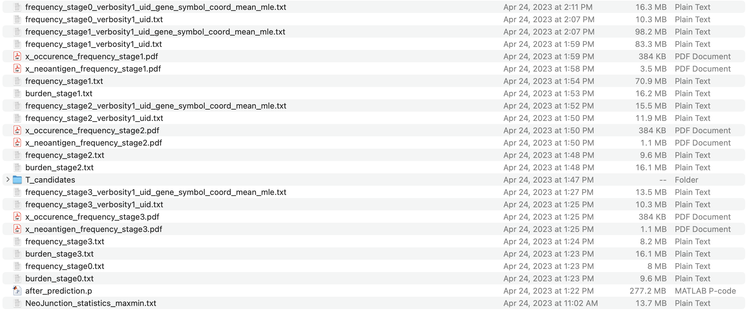
NeoJunction_statistics_maxmin.txt contains the filtering step regarding how each junctions were either filered out or retained by each control database. For each stage, it means different
steps in the neoantigen production:
stage 0: neojunction, the number of tumor-specific junction readsstage 1: peptides that are predicted (3-way in-silico translation) from each neojunctionstage 2: peptides that are predicted to be presented on an MHC molecule (based on netMHCpan or MHCflurry prediction)stage 3: peptides that are predicted to be immunogenic (DeepImmuno)
For each stage, you may see the following categories of results:
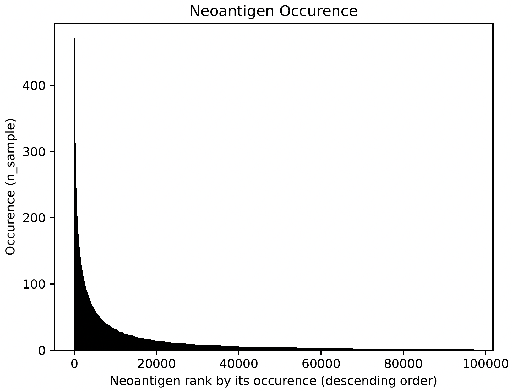
burden_stage{0-3}.txt: This file characterizes the patient level neoantigen burden (See below concrete example).frequency_stage{0-3}.txt: This file chracterizes each specific neoantigen, how many times does it occur across the whole cohort?frequency_stage{0-3}_verbosity1_uid_gene_symbol_coord_mean_mle.txt: This is an enhanced version of frequency.txt file.x_neoantigen_frequency{0-3}.pdf: This is a visual representation of neoantigen frequency as a sorted barplot, where each bar is a neoantigen and the height is its occurence across cohorts.x_occurence_frequency{0-3}.pdf: This is an alternative visualization of neoantigen frequency as a histplot, interval (x-axis) with the occurence of each neoantigen across the cohort.
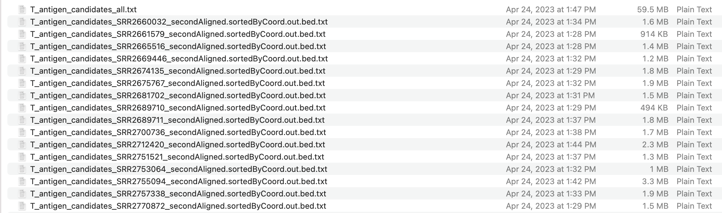
For the final immunogenic neoantigen, we have detailed reports in T_candidates folder (amplify the webpage to see more clearly), here each row represent
a peptide-HLA combination, so that binding affinity and immunogenicity are also reported. See Troubleshooting page for more detailed explanation for the output file in
T_candidates folder.
The burden matrix should look like the below, where the last column and last row represent the mean burden for each feature and the total burden for each sample. Since this output only illustrates the last 10 columns and rows, all of the entries are zero, to give the user a sense of the file layout.
TCGA-DA-A3F3-06A-11R-A20F-07.bed |
TCGA-EE-A3JI-06A-11R-A21D-07.bed |
TCGA-EE-A2GU-06A-11R-A18T-07.bed |
TCGA-EE-A2GB-06A-11R-A18T-07.bed |
TCGA-EE-A29N-06A-12R-A18S-07.bed |
TCGA-FS-A1ZK-06A-11R-A18T-07.bed |
TCGA-EE-A3AG-06A-31R-A18S-07.bed |
TCGA-EE-A2GD-06A-11R-A18T-07.bed |
TCGA-EE-A2MD-06A-11R-A18T-07.bed |
mean |
|
|---|---|---|---|---|---|---|---|---|---|---|
ENSG00000112208:E1.1-E2.1 |
0.0 |
0.0 |
0.0 |
0.0 |
0.0 |
0.0 |
0.0 |
0.0 |
0.0 |
0.0 |
ENSG00000112200:E6.1-E10.1 |
0.0 |
0.0 |
0.0 |
0.0 |
0.0 |
0.0 |
0.0 |
0.0 |
0.0 |
0.0 |
ENSG00000112200:E20.1-E21.2 |
0.0 |
0.0 |
0.0 |
0.0 |
0.0 |
0.0 |
0.0 |
0.0 |
0.0 |
0.0 |
ENSG00000112200:E2.11-E3.3 |
0.0 |
0.0 |
0.0 |
0.0 |
0.0 |
0.0 |
0.0 |
0.0 |
0.0 |
0.0 |
ENSG00000112200:E2.11-E3.2 |
0.0 |
0.0 |
0.0 |
0.0 |
0.0 |
0.0 |
0.0 |
0.0 |
0.0 |
0.0 |
ENSG00000112200:E19.2-E20.1 |
0.0 |
0.0 |
0.0 |
0.0 |
0.0 |
0.0 |
0.0 |
0.0 |
0.0 |
0.0 |
ENSG00000112200:E18.1-E19.2 |
0.0 |
0.0 |
0.0 |
0.0 |
0.0 |
0.0 |
0.0 |
0.0 |
0.0 |
0.0 |
ENSG00000112200:E17.1-E18.1 |
0.0 |
0.0 |
0.0 |
0.0 |
0.0 |
0.0 |
0.0 |
0.0 |
0.0 |
0.0 |
ENSG00000125676:E31.2-E32.1 |
0.0 |
0.0 |
0.0 |
0.0 |
0.0 |
0.0 |
0.0 |
0.0 |
0.0 |
0.0 |
burden |
5601.0 |
5641.0 |
5653.0 |
5693.0 |
5716.0 |
5949.0 |
6222.0 |
6418.0 |
6700.0 |
2858.5 |
Neoantigen frequency plot shows the distinctive pattern between shared neoantigens (left part) and unique neoantigens (right part).
Interface to proteomics validation
Now imagine we have a handful of predicted short-peptides that potentially can be therapeutically valuable targets, as a routine step, we definitely want to test whether they are supported by public or in-house MS (either untargeted or targetted HLA-bound immunopeptidome) datasets. We provide a set of functions that can make this validation process easier.
First, we want to extract all candidate and write them into a fasta file, we iterate all the samples in a for loop, we remove the identical peptides, becasue same peptide can be generated from different junctions. Next, we want to remove all peptides that are overlapping with human proteome, you can download any preferred human proteome database (UCSC or Uniprot), we provide a reference fasta human_uniprot_proteome.fasta downloaded from Uniprot downloaded at Jan 2020, available at SNAF GitHub, we chop them into 9 and 10 mers without duplicates. Then we remove overlapping candidates, all the above is like below:
jcmq = snaf.JunctionCountMatrixQuery.deserialize('result/after_prediction.p')
os.mkdir('./fasta')
snaf.chop_normal_pep_db(fasta_path='../SNAF_ecosystem/snaf_aux/human_uniprot_proteome.fasta',output_path='./fasta/human_proteome_uniprot_9_10_mers_unique.fasta',mers=[9,10],allow_duplicates=False)
for sample in df.columns:  # df is the counts.original.pruned.txt file
    jcmq.show_neoantigen_as_fasta(outdir='./fasta',name='neoantigen_{}.fasta'.format(sample),stage=3,verbosity=1,contain_uid=True,sample=sample)
    snaf.remove_redundant('./fasta/neoantigen_{}.fasta'.format(sample),'./fasta/neoantigen_{}_unique.fasta'.format(sample))
    snaf.compare_two_fasta(fa1_path='./fasta/human_proteome_uniprot_9_10_mers_unique.fasta',
                        fa2_path='./fasta/neoantigen_{}_unique.fasta'.format(sample),outdir='./fasta',
                        write_unique2=True,prefix='{}_'.format(sample))
The above assume we want to validate the immunogenic neoantigens (stage 3) identified for each patients. You can certainly construct other fasta files
based on the SNAF-T output, and optionally use the auxiliary functions (remove_redundant and compare_two_fasta) to remove redundant peptides and overlapping peptides.
Usually, MS software requires a customized fasta database, you’ve already had that right now. Depending on which MS software you use, the configuration steps can vary, but we recommend using MaxQuant here which is highly regarded. MaxQuant requires to compile a configuration files called mqpar.xml which stores the setting for the search engine, we provide a programatical API to modify the config file based on different instrument, database and raw files you are using, below is using Thermo Orbitrap:
dbs = ['/data/salomonis2/LabFiles/Frank-Li/neoantigen/MS/schuster/RNA/snaf_analysis/fasta/SRR5933726.Aligned.sortedByCoord.out.bed_unique2.fasta',
       '/data/salomonis2/LabFiles/Frank-Li/neoantigen/MS/human_uniprot_proteome.fasta']
inputs = ['/data/salomonis2/LabFiles/Frank-Li/neoantigen/MS/schuster/MS/OvCa48/OvCa48_classI_Rep#1.raw',
          '/data/salomonis2/LabFiles/Frank-Li/neoantigen/MS/schuster/MS/OvCa48/OvCa48_classI_Rep#2.raw',
          '/data/salomonis2/LabFiles/Frank-Li/neoantigen/MS/schuster/MS/OvCa48/OvCa48_classI_Rep#3.raw']
outdir = '/data/salomonis2/LabFiles/Frank-Li/neoantigen/MS/schuster/MS/OvCa48'
snaf.proteomics.set_maxquant_configuration(base='/path/to/download/mqpar.xml',dbs=dbs,n_threads=20,inputs=inputs,enzymes=None,enzyme_mode=4,protein_fdr=1,peptide_fdr=0.05,site_fdr=1,
                                           outdir=outdir,minPepLen=8,minPeptideLengthForUnspecificSearch=8,maxPeptideLengthForUnspecificSearch=11)
Warning
For the above, even just one file path, please still use list. Second, please use absolute path to avoid maxquant error. Third, see troubleshooting page for how to run MaxQuant on Linux.
The
outdirshould be folder where all your .raw or .d file/folder sit.The above parameters just represent a suggestions not a fixed requrement. For discovery analysis, I tent to set
peptide_fdr=1to give the software best chance to find the peptides then gradually descrease the FDR to see how the results change. Alternative metrics I considered before are MaxQuant-returnedAndromedata score>40andPosterior Error Probability (PEP)<0.01when evaluating whether a peptide-spectrum match worth validating or not. I have seen hundreds of high-confidence peptides reported by other proprietory softwares (ProteomeDiscovery, PEAKS, Byonic) that didn’t pass MaxQuant FDR cutoff or reported as low score, this issue has been reported by other users as well (issue1, issue2, issue3).In the manuscript, I also tried to not including human proteome but search directly against the neoantigen database, in this context, you should set
enzyme_mode=5(no digestion). This inherently subject to false positive but can also be informative, because the searching will be calibrated specifically for short, non-trypic peptides.
Above, we need a base ‘mqpar.xml’ file to modify upon, we provide a few base files.
For folks who are not familiar with MaxQuant, Here I provided the MaxQuant 2.0.3.1 just download the whole
folder, and then you just use the v2.0.3.1 base mqpar.xml provided in the GitHub. Follow the troubleshooting page on how to run MaxQuant on Linux server.
Alternatively, if you are familiar with MaxQuant, you can download the latest version from their official
website, using your windows PC to configure a mqpar.xml file. If your MS raw files are not in these formats (e.g. orbitrap FAMIS), you can either contact me or just follow the MaxQuant GUI instructions. A automatically generated configuration
file (mqpar.xml) will be shown in the outdir that you specified. More information can be found in the Interface to proteomics.
Visualization
A very important question users will want to ask is what splicing event produces a certain neoepitope? We provide a convenient plotting function to achieve this, usually we want to first deserialize the resultant pickle object back to memory from last step:
jcmq = snaf.JunctionCountMatrixQuery.deserialize('result/after_prediction.p')
jcmq.visualize(uid='ENSG00000167291:E38.6-E39.1',sample='TCGA-DA-A1I1-06A-12R-A18U-07.bed',outdir='./result')
Warning
For all the visualization functions, you still need to load all the required global variable by first initializing SNAF, so the initialization code should precede the visualization code, see this issue for more detail..

It is also quite important to know the tumor specificity of each junction, which can be visualized in various ways as below:
# interactive
snaf.gtex_visual_combine_plotly(uid=uid,outdir='result_new/common',norm=False,tumor=df)
# static
dff = snaf.gtex_visual_combine(uid=uid,outdir='Frank_inspection',norm=False,tumor=df,group_by_tissue=False)


Survival Analysis
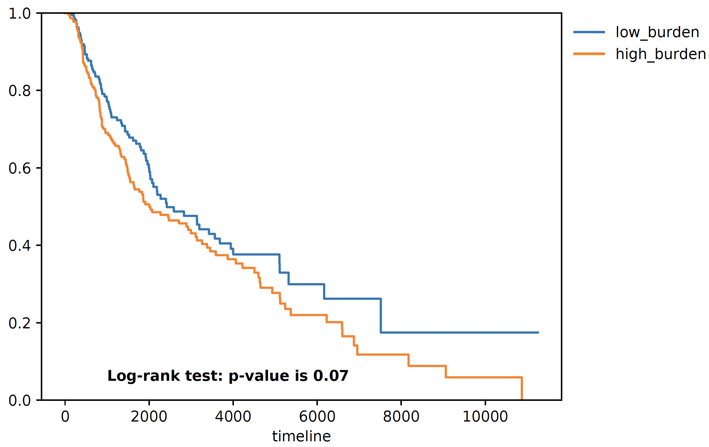
We download the TCGA SKCM survival data from Xena browser, we provide a convenient function to do a survival analyis using various stratification criteria, To use this function, we need a dataframe (survival) whose index is sample name, along with two columns one representing event (OS.death) and one representing duration (OS.time). Another is burden, it is a pandas dataframe generated by SNAF-T, with sample name as index. The sample name needs to be the same, that’s why we need a few lines of code for parsing below:
survival = pd.read_csv('TCGA-SKCM.survival.tsv',sep='\t',index_col=0)  # 463
burden_df = pd.read_csv('burden_stage2.txt',sep='\t',index_col=0)
burden_df.rename(columns=lambda x:'-'.join(x.split('-')[:4]),inplace=True)
# convenient function for survival, and save the output for whether a sample is in which group (high, low)
burden_output, _ = snaf.survival_analysis(burden_df,survival,n=2,stratification_plot='result/stage2_stratify.pdf',survival_plot='result/stage2_survival.pdf')
burden_output.to_csv('result/sample_to_burden_group.txt',sep='\t')
We can also perform Cox regression analysis to see if the precense of a particular neoantigne is associated with survival or not, it can also be whether the
presence of a neoantigen is associated with responding to immunotherapy or not, here the rename function is to convert the sample name from your freq file
to the sample name in survival file, the pea is the path to a file usually located at your altanalyze_output/AltResults/AlternativeOutput folder called
Hs_RNASeq_top_alt_junctions-PSI_EventAnnotation.txt, the mode is either binary or psi, it dictates whether to just binarize (presence or absence) of
a junction or use the junction presence level as well:
snaf.downstream.survival_regression(freq='result_new/frequency_stage3_verbosity1_uid_gene_symbol_coord_mean_mle.txt',remove_quote=True,
                                    rename_func=lambda x:'-'.join(x.split('-')[:4]),survival='TCGA-SKCM.survival.tsv',
                                    pea='Hs_RNASeq_top_alt_junctions-PSI_EventAnnotation.txt',outdir='result_new/survival',mode='binary')
uid |
pep |
junc |
n_valid_sample |
wald_z_score |
wald_p_value |
|---|---|---|---|---|---|
YGQSAFHYL,ENSG00000135903:E10.3-E11.1 |
YGQSAFHYL |
ENSG00000135903:E10.3-E11.1 |
409 |
1.235222144 |
0.21674784 |
TTMPSSQVL,ENSG00000164175:E2.3-E3.2 |
TTMPSSQVL |
ENSG00000164175:E2.3-E3.2 |
381 |
1.807299623 |
0.070715575 |
GSMDKVPFI,ENSG00000135903:E10.3-E11.1 |
GSMDKVPFI |
ENSG00000135903:E10.3-E11.1 |
379 |
0.523009106 |
0.600967916 |
SLYSYFQKV,ENSG00000164175:E5.3-E6.2 |
SLYSYFQKV |
ENSG00000164175:E5.3-E6.2 |
378 |
2.216503829 |
0.026657016 |
HAEQTRRAM,ENSG00000164175:E3.4-E4.2 |
HAEQTRRAM |
ENSG00000164175:E3.4-E4.2 |
376 |
1.800910433 |
0.071716998 |
YFQKVLVSY,ENSG00000164175:E5.3-E6.2 |
YFQKVLVSY |
ENSG00000164175:E5.3-E6.2 |
358 |
2.267340259 |
0.023369448 |
SVFSSLYSY,ENSG00000164175:E5.3-E6.2 |
SVFSSLYSY |
ENSG00000164175:E5.3-E6.2 |
352 |
2.70980595 |
0.006732258 |
SYPQIQNNL,ENSG00000180318:E3.1-E4.1 |
SYPQIQNNL |
ENSG00000180318:E3.1-E4.1 |
352 |
0.165661834 |
0.868423083 |
TGFGGALGY,ENSG00000164175:E2.3-E3.2 |
TGFGGALGY |
ENSG00000164175:E2.3-E3.2 |
351 |
2.501555124 |
0.012364919 |
Differential Gene/Splicing Analysis and Gene Enrichment analysis
We can ask the questions, what are the differentially up-regulated or down-regulated genes and splicing events in high splicing burden patients compared to low burden group. And even further, for those up-regulated genes, what are the enriched pathway/ontology for these genes.
To run differential gene or splicing analysis, we need to create a groups.txt file and a comps.txt file as below, both are tab delimited and
no header line, the groups file specifiy the label of each sample, third column is the label and the second column is just a numerical of the label, and the
comps file is just one line with 1,tab,2,newline:
# groups.task.txt file
sample_1    1    high
sample_2    1    high
sample_3    1    high
...        ...    ...
sample_n    2     low

# comps.task.txt file
1   2
Once you have these two files, you can run Differential anlaysis first using the docker again, please pay special attention to how the folder structure look like:
bam/
bed/
altanalyze_output/
    AltAnalyze_report-20231007-154042.log
    AltResults/
    ExpressionInput/
    AltDatabase/
    DataPlots/
    ExpressionOutput/
    AltExpression/
    ExonPlots/
    GO-Elite/
groups.task.txt
comps.task.txt
Imagining the above is your current folder ($PWD), Now you can run the following commands:
# using singularity
singularity run -B $PWD:/mnt --writable /path/to/altanalyze/ DE altanalyze_output groups.txt  # differential gene
singularity run -B $PWD:/mnt --writable /path/to/altanalyze/ DAS altanalyze_output groups.txt   # differential splicing

# using docker
docker run -v $PWD:/mnt frankligy123/altanalyze:0.7.0.1 DE altanalyze_output groups.txt  # differential gene
docker run -v $PWD:/mnt frankligy123/altanalyze:0.7.0.1 DAS altanalyze_output groups.txt   # differential splicing
After running that, your DEG results should be a file in altanalyze_output/ExpressionInput/DEGs-LogFold_0.0_adjp/GE.high_vs_low.txt, the differential
splicing results should be a file in altanalyze_output/AlternativeOutput/Events-dPSI_0.0_rawp/PSI.high_vs_low.txt. Once you have those files, you can use the
convenient visualization function to generate routine visualization:
# plot volcano
snaf.downstream.visualize_DEG_result('result_new/survival/DEGs-LogFold_0.0_adjp/GE.low_vs_high_mod.txt',up_cutoff=0.58,down_cutoff=-0.58,
                                      mode='static',outdir='result_new/survival',genes_to_highlight=['LST1','HCST','IL32','CD3D','S100A8','MZB1','IGLC4','ADAM10','ARFGEF2','MIB1','KIF3B','TNPO1','PTPN11','ANKRD52','TGFBR1'])

Further, you can examine the different splicing event types:
# Event type difference
psi = pd.read_csv('PSI.grow_vs_senes.txt',sep='\t',index_col=0)
uid_in_exp = [':'.join(item.split('|')[0].split(':')[1:]) for item in psi.loc[(psi['dPSI']<0)&(psi['adjp']<0.05),:].index.tolist()]
uid_in_ctl = [':'.join(item.split('|')[0].split(':')[1:]) for item in psi.loc[(psi['dPSI']>0)&(psi['adjp']<0.05),:].index.tolist()]
snaf.plot_event_type(pea='Hs_RNASeq_top_alt_junctions-PSI_EventAnnotation.txt',uids={'exp':uid_in_exp,'ctl':uid_in_ctl},rel=True,outdir='./')

Finally, you can conduct gene enrichment analysis by first extract the top marker genes from your DE analysis above, we just need a gene_list.txt file as below:
# gene_list.txt file
gene1
gene2
...
gene_n
This will create a gene_list file to extract genes that fullfil the cutoffs you set, and write to the outdir you set, now for illustration purpose,
imagine you copy the gene_list file to the folder where altanalyze_output folder sits from first step, and you are now in this folder:
# using singularity
singularity run -B $PWD:/mnt --writable /path/to/altanalyze/ GO gene_list.txt

# using docker
docker run -v $PWD:/mnt frankligy123/altanalyze:0.7.0.1 GO gene_list.txt
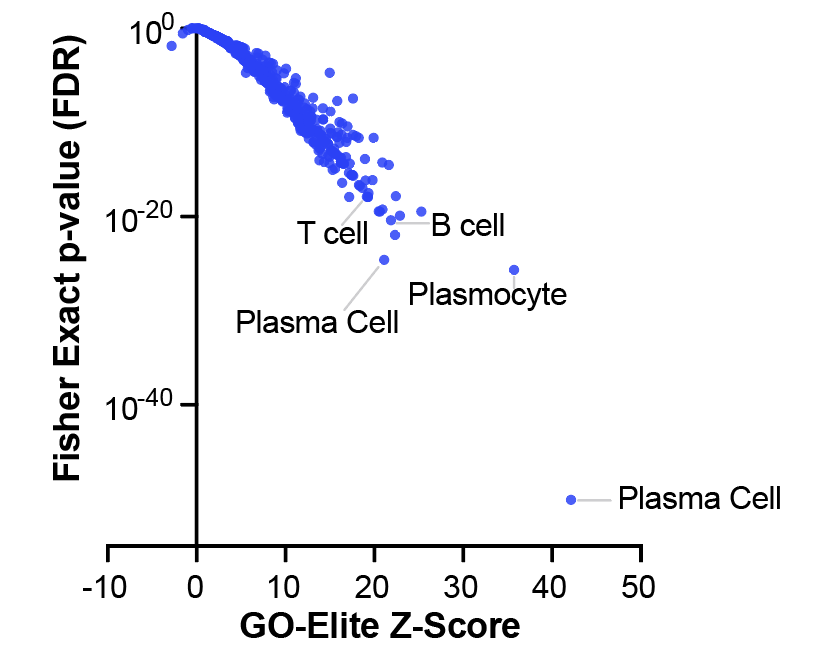
You should have two folders, one called GO_Elite_result_BioMarkers and another called GO_Elite_result_GeneOntology, the first one contains
enriched biomarkers for cell type or published papers, second one contains enriched ontologies. The actual files are at GO_Elite_result_BioMarkers/GO-Elite_results/CompleteResults/ORA/archived-{time_stamp}/gene_list-BioMarkers.txt
and GO_Elite_result_GeneOntology/GO-Elite_results/CompleteResults/ORA/archived-{time_stamp}/gene_list-GO.txt, we again provide a visualization function:
# plot enrichment
snaf.downstream.visualize_GO_result(path_list=['result_new/survival/GO_Elite_result_BioMarkers/GO-Elite_results/CompleteResults/ORA/archived-20230528-192111/gene_list_up_in_low-BioMarkers.txt','result_new/survival/GO_Elite_result_GeneOntology/GO-Elite_results/CompleteResults/ORA/archived-20230528-192137/gene_list_up_in_low-GO.txt'],
                                    skiprows_list=[16,17],category_list=['Gene-Set Name','Ontology Name'],outdir='result_new/survival',
                                    mode='static',ontology_to_highlight={'Adult Peripheral Blood Activated T cell (PMID32214235 top 100)':'T cells','antigen binding':'antigen binding','complement activation':'Complement Activation','immune response':'immune response','humoral immune response':'humoral immune response'},ylims=(10e-85,10e-1))
Mutation Association Analysis
We download the TCGA SKCM mutation data from <Xena browser>. We provide a convenient function to calculate all associations and plot them. To explain how
this function work, basically, it has two mode, compute mode is to compute the association between each gene mutation and neoantigen burden. plot mode
is to visualize selective genes as a side-by-side barplot. For compute mode, we need the burden file (again, a pandas series, same as described above in survival analysis),
and mutation, which is a dataframe whose index is sample name, and one column represents mutated gene. For plot mode, just need to specify a list of
genes to plot:
mutation = pd.read_csv('TCGA-SKCM.mutect2_snv.tsv',sep='\t',index_col=0)  # 467 samples have mutations
mutation = mutation.loc[mutation['filter']=='PASS',:]
burden = pd.read_csv('result/burden_stage3.txt',sep='\t',index_col=0).loc['burden',:].iloc[:-1]  # 472
burden.index = ['-'.join(sample.split('-')[0:4]) for sample in burden.index]
# mutation convenience function, compute mode
snaf.mutation_analysis(mode='compute',burden=burden,mutation=mutation,output='result/stage3_mutation.txt',gene_column='gene')
# mutation convenience function, plot mode
snaf.mutation_analysis(mode='plot',burden=burden,mutation=mutation,output='result/stage3_mutation_CAMKK2.pdf',genes_to_plot=['CAMKK2'])
mutation_gene |
n_samples |
pval |
adjp |
|---|---|---|---|
OGFOD3 |
13 |
3.82E-05 |
0.272783716 |
CAMKK2 |
19 |
5.25E-05 |
0.272783716 |
ACE |
56 |
0.00305804 |
0.357487136 |
PALMD |
22 |
0.003794017 |
0.357487136 |
CEP350 |
35 |
0.001240149 |
0.357487136 |
PROM2 |
50 |
0.000457734 |
0.357487136 |
STAT4 |
40 |
0.003968346 |
0.357487136 |
DOCK10 |
24 |
0.000289835 |
0.357487136 |
QARS |
12 |
0.000546601 |
0.357487136 |
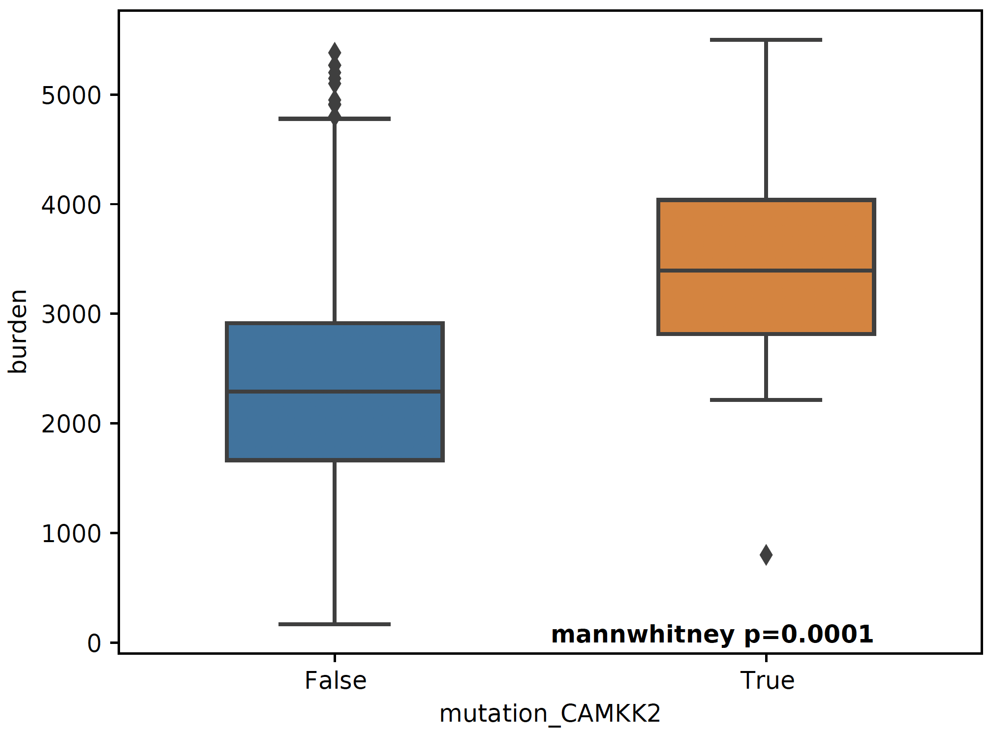
For a specific mutation CAMKK2, which has been reported that the suppresses expression of this gene, which can increase ferroptosis efficacy and
anti-PD1 immunotherapy (paper link), we show that patients with mutated CAMKK2 have higher
neoantigen burden so that can explain why it lead to better immunotherapy efficacy.
Interactive Neoantigen Viewer
Users can launch a dash interactive neoantigen viewer to visualize all the neoantigens based on their physiochemical properties and their motif
composition along with the source splicing junction. To achieve it, we first run a pre-processing step analyze_neoantigens to generate
some portable input file for the viewer, we need a file named shared_vs_unique_neoantigen_all.txt. Be sure the specify the full name for this file,
also, the umap plot may take 10 seconds to load if you don’t see it loads instantly:
snaf.analyze_neoantigens(freq_path='result/frequency_stage2_verbosity1_uid.txt',junction_path='result/burden_stage0.txt',total_samples=2,outdir='result',mers=None,fasta=False)
snaf.run_dash_T_antigen(input_abs_path='/data/salomonis2/LabFiles/Frank-Li/neoantigen/TCGA/SKCM/snaf_analysis/result/shared_vs_unique_neoantigen_all.txt')

Identify altered surface proteins (B-antigen)
As a separate workflow, the B-antigen pipeline aims to priotize the altered surface protein from abnormal splicing events.
Instantiating B pipeline
We should copy the first part of T antigen pipeline and add additional initialization step for surface antigen:
import os,sys
import pandas as pd
import numpy as np
import anndata as ad
import snaf

# copy the first part of T antigen pipeline

# read in the splicing junction matrix
df = pd.read_csv('/user/ligk2e/altanalyze_output/ExpressionInput/counts.original.pruned.txt',index_col=0,sep='\t')
# database directory (where you extract the reference tarball file) and netMHCpan folder
db_dir = '/user/ligk2e/download'
netMHCpan_path = '/user/ligk2e/netMHCpan-4.1/netMHCpan'
# demonstrate how to add additional control database, see below note for more
tcga_ctrl_db = ad.read_h5ad(os.path.join(db_dir,'controls','tcga_matched_control_junction_count.h5ad'))
gtex_skin_ctrl_db = ad.read_h5ad(os.path.join(db_dir,'controls','gtex_skin_count.h5ad'))
add_control = {'tcga_control':tcga_ctrl_db,'gtex_skin':gtex_skin_ctrl_db}
# initiate
snaf.initialize(df=df,db_dir=db_dir,binding_method='netMHCpan',software_path=netMHCpan_path,add_control=add_control)

# additional instantiation steps
from snaf import surface
surface.initialize(db_dir=db_dir)
Running the program
We first obtain the membrane splicing events:
membrane_tuples = snaf.JunctionCountMatrixQuery.get_membrane_tuples(df,add_control=add_control,outdir='result_new/surface')
There are two modes for running B-pipeline, one is de novo prediction of full isoform from short-read, and validate those prediction by providing an additional long-read gtf.
Alternatively, you can use one of our internal pan-cancer long-read isoform database to predict the full-length isoform. The former is called short_read mode, the latter is called
long_read mode. The below referred gtf files can be downloaded from this synapse folder:
# short_read mode
surface.run(uids=membrane_tuples,outdir='result/surface',prediction_mode='short_read',
            gtf=None,
            tmhmm=True,software_path='/data/salomonis2/LabFiles/Frank-Li/python3/TMHMM/tmhmm-2.0c/bin/tmhmm')
surface.generate_full_results(outdir='result/surface',mode='short_read',
                              freq_path='result/frequency_stage0_verbosity1_uid_gene_symbol_coord_mean_mle.txt',
                              validation_gtf='/data/salomonis2/LabFiles/Frank-Li/neoantigen/TCGA/SKCM/snaf_analysis/SQANTI-all/collapse_isoforms_classification.filtered_lite.gtf')


# long_read mode
surface.run(uids=membrane_tuples,outdir='result/surface',prediction_mode='long_read',
            gtf='/data/salomonis2/LabFiles/Frank-Li/refactor/data/2021UHRRIsoSeq_SQANTI3_filtered.gtf',
            tmhmm=True,software_path='/data/salomonis2/LabFiles/Frank-Li/python3/TMHMM/tmhmm-2.0c/bin/tmhmm')
surface.generate_full_results(outdir='result/surface',mode='long_read',
                              freq_path='result/frequency_stage0_verbosity1_uid_gene_symbol_coord_mean_mle.txt',
                              validation_gtf=None)
You can refer to GitHub Issue 35 for how to construct your own custom GTF/GFF for long-read data.
In your result folder, if running short_read mode, you will be able to get following results (amplify the webpage to see more clearly):
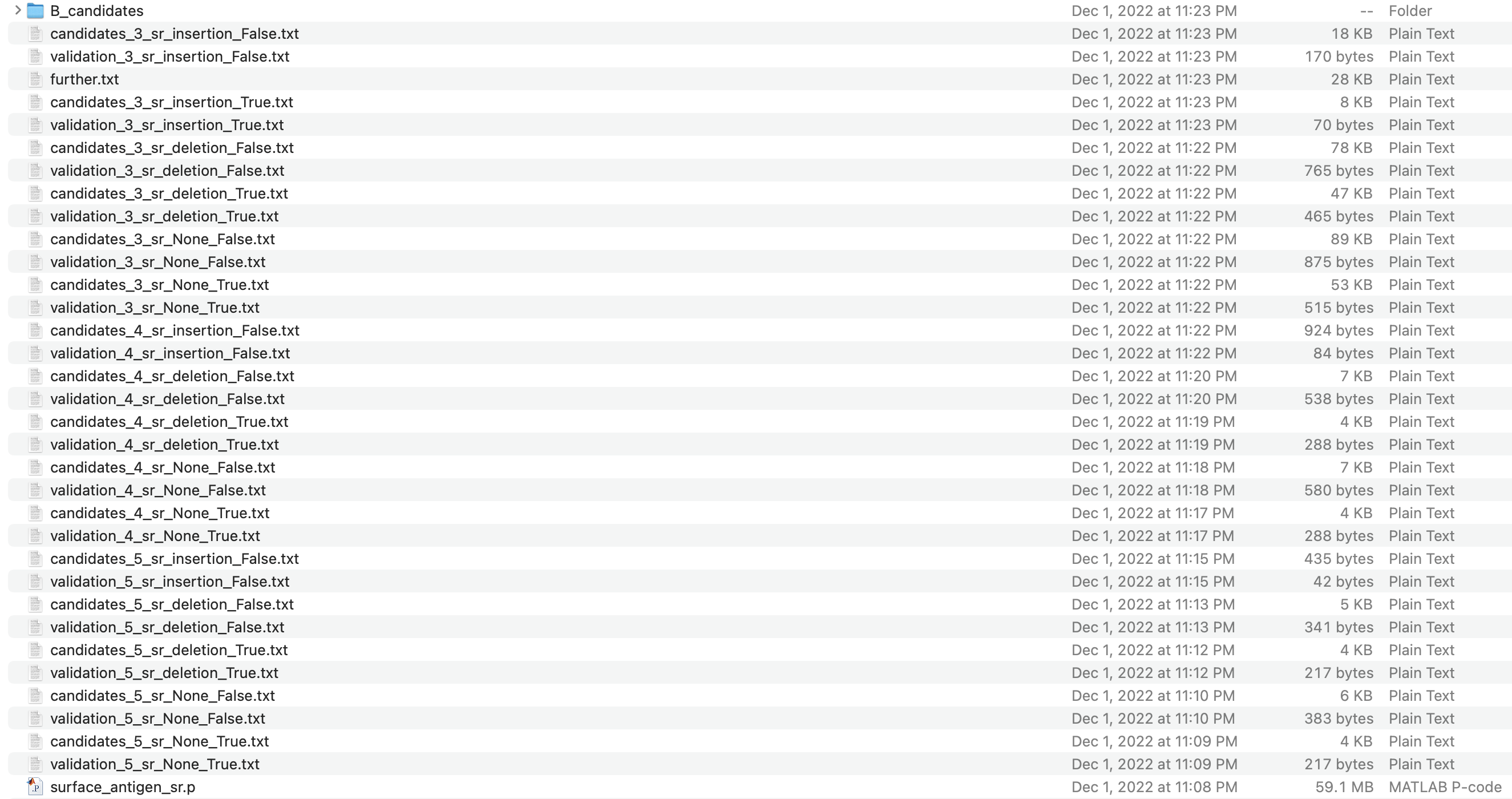
Different strigencies are explanined below:
strigency 1: The novel isoform needs to be absent in UniProt databasestrigency 2: The novel isoform also needs to be a documented protein-coding genestrigency 3: The novel isoform also needs to not be subjected to Nonsense Mediated Decay (NMD)strigency 4: The novel isoform also needs to have long-read or EST support (as long as the novel junction present in full-length)strigency 5: The novel isoform also needs to have long-read or EST support (whole ORF needs to be the same as full-length)
An output called candidates.txt is what we are looking for, to facilitate the inspection of the result, let’s use the B antigen viewer shown below. Also,
we automatically generate a more readable and publication-quality table for each category of candidates by using report_candidates.
Particurly, a more human-readable results can be found in B_candidates folder, you should examine a file named sr_str3_report_None_False.txt which is a superset for other output,
str controls the strigency, deletion/insertion/None indicate whether the candidate has deleted or inserted neo-epitope, None is the combination of both. False/True represents whether
the candidate will be extracellular or not, False is the superset of True.
Warning
The prediction for extracellular and intracellular is subject to false prediction, due to complexity of altered topology. The program basically intersected the junction region with the documented extracellular regions, but for multiple Transmembrane protein with drastically disrupted topology, it is hard to precisely define. Further inspection using B-Viewer, Protter and Alphafold2 would be beneficial.
The long-read mode output is similar and the file names should be self-explanable if you can follow the above clarificaitons. Basically you should be looking for
a file named lr_str3_report_None_False.txt for human readable result, and candidates_3_lr_None_False.txt for using B-antigen Viewer as shown below.
Interactive neoantigen viewer
Similar to T antigen, users can explore all the altered surface protein for B antigen, we need the pickle object and the candidates file,
importantly, please specify the full path to the python executable you use to run your python script, below using long_read mode result as an example:
surface.run_dash_B_antigen(pkl='result/surface/surface_antigen_lr.p',candidates='result/surface/candidates_3_lr_None_False.txt',
                           prediction_mode='long_read',
                           python_executable='/data/salomonis2/LabFiles/Frank-Li/refactor/neo_env/bin/python3.7')
Note
The reason for specifying python_executable is for using EmBoss Needleman global alignment REST API. As the REST API was provided as a python script, I need the python executable full path to execute the script.

Compatibility (Gene Symbol & chromsome Coordinates & Genome Version)
For some historical reasons, different RNA splicing pipeline (i.e. AltAnalyze, MAJIQ, rMATs, LeafCutter, etc) use their own gene model, meaning how they define and index gene and exon number. Hence, a splicing junction (chromsome coordinate like chr7:156999-176000) maybe reprensented in diverse annotation in different pipelines.
It is in our to-do list but also requires a lot of work to harmonize all the annotations, for now, we provide functions to convert AltAnalyze annotation
to the most generic representation, namely, gene symbol and chromosome coordinates. It will be handled by two functions, Add gene symbol and Add chromsome coordinate.
And in the latest version, an enhanced version of frequency tables will be automatically generated. Below is just for illustration purpose.
Regarding the Genome Version, The best practice now is to use hg38 aligned bam file to run SNAF, utilizing the richest and well-evaluated reference database
we curated. Then users can use liftover program downloadable from UCSC genome browser to lift the junction coordinate from one to the other. From my experience,
despite certain false conversion, most of the time the conversion is very accurate.
Now let’s take the output frequency_stage2_verbosity1_uid.txt as the example (most important thing is pandas dataframe index format):
                                                  n_sample
TQLSVPWRL,ENSG00000258017:E2.3-E2.6                  470
QIFESVSHF,ENSG00000198034:E8.4-E9.1                  463
MGSKRLTSL,ENSG00000241343:E2.2-E2.4                  449
HALLVYPTL,ENSG00000090581:E5.10-E5.24                    435
QFADGRQSW,ENSG00000111843:E9.1-ENSG00000137210:E6.1  433
GIHPSKVVY,ENSG00000263809:E3.1-E4.1                  432
RPYLPVKVL,ENSG00000134330:E8.4-E9.1                  432
LPPPRLASV,ENSG00000090581:E5.10-E5.24                    428
SSQVHLSHL,ENSG00000172053:E11.8-E11.11                   425
Let’s add gene symbol to the dataframe:
df = snaf.add_gene_symbol_frequency_table(df=df,remove_quote=True)
Note
The remove_quote argument is due to the fact that in frequency.txt file, one column is the list of all sample names that contain
the splicing neoantigen. The thing is, when such a list being re-read into the memory, sometimes a quotation will be added so that the data type
become a string instead of list, which is not desirable, so if your df is read using pd.read_csv, you need to set it as True,
otherwise, set it as False.
The resultant will look like that:
                                                 n_sample                   symbol
TQLSVPWRL,ENSG00000258017:E2.3-E2.6                 470                    unknown_gene
QIFESVSHF,ENSG00000198034:E8.4-E9.1                 463                         RPS4X
MGSKRLTSL,ENSG00000241343:E2.2-E2.4                 449                        RPL36A
HALLVYPTL,ENSG00000090581:E5.10-E5.24                   435                     GNPTG
QFADGRQSW,ENSG00000111843:E9.1-ENSG00000137210:E6.1 433                        TMEM14C
GIHPSKVVY,ENSG00000263809:E3.1-E4.1                 432                     unknown_gene
RPYLPVKVL,ENSG00000134330:E8.4-E9.1                 432                         IAH1
LPPPRLASV,ENSG00000090581:E5.10-E5.24                   428                    GNPTG
SSQVHLSHL,ENSG00000172053:E11.8-E11.11                  425                    QARS1
Let’s add chromsome coorinates to the splicing junction annotation as well:
df = snaf.add_coord_frequency_table(df=df,remove_quote=False)
Results look like this:
                                                    n_sample                   symbol                coord
TQLSVPWRL,ENSG00000258017:E2.3-E2.6                   470              unknown_gene    chr12:49128207-49128627(+)
QIFESVSHF,ENSG00000198034:E8.4-E9.1                   463                  RPS4X       chrX:72256054-72272640(-)
MGSKRLTSL,ENSG00000241343:E2.2-E2.4                   449                  RPL36A      chrX:101391235-101391459(+)
HALLVYPTL,ENSG00000090581:E5.10-E5.24                     435                      GNPTG       chr16:1362320-1362452(+)
QFADGRQSW,ENSG00000111843:E9.1-ENSG00000137210:E6.1   433                 TMEM14C      chr6:10728727-10756467(+)
GIHPSKVVY,ENSG00000263809:E3.1-E4.1                   432               unknown_gene        chr17:8376104-8379796(-)
RPYLPVKVL,ENSG00000134330:E8.4-E9.1                   432                   IAH1        chr2:9484550-9487456(+)
LPPPRLASV,ENSG00000090581:E5.10-E5.24                     428                       GNPTG       chr16:1362320-1362452(+)
SSQVHLSHL,ENSG00000172053:E11.8-E11.11                    425                       QARS1      chr3:49099853-49099994(-)